1. Gradient descent optimization
Gradient-based methods make use of the gradient information to adjust the parameters. Among them, gradient descent can be the simplest. Gradient descent makes the parameters to walk a small step in the direction of the negative gradient.
$$ \mathbf{w}^{\tau + 1} = \mathbf{w}^{\tau} - \eta \nabla_{\mathbf{w}^{\tau}} E \tag{1.1} $$
where \(\eta, \tau, E\) label learning rate (\(\eta > 0\)), the iteration step and the loss function.
Wait! But why is the negative gradient?
2. Why negative gradient
The function increases the most sharply by following the direction of the gradient.
The below is an example. The three-dimensional plane is \(z = F(x, y)\). The black point is on the plane. You can try to move the point to see how the arrow changes. Interestingly, the arrow always points to the direction which leads to the biggest increase of the function value. Note that when you move one step, the gradient just changes. Thus if you still want to increase the function value in the most sharp way, another computation is needed.
The starting point of the arrow is the mapping of the black point to the \(xoy\) plane. The arrow is parallel to the gradient.
the illustration of the direction of gradient
Let us use another graph to better understand what the mapping means. The left graph is contour plot while the right is the plane. The red point is just the mapping of the black point to $xoy$ plane. The blue arrow is just the direction of the gradient. And you can move the point to feel about it.
another illustration
That is the intuitive way to feel about the gradient. Furthermore, we can just try to prove it.
Consider a Taylor Expansion:
When you decide to move a small step, the two magnitudes are certain. If $\theta=0$, you can maximize the function value (i.e. in the direction of the gradient).
Thus if we want to minimize our loss function, we need to go in the opposite direction of the gradient. That is why we need a negative gradient. Also, note that Taylor Expansion only applies to small \(\Delta x\) which further requires \(\eta\) to be small (e.g. \(2 \times 10^{-5}, 5 \times 10^{-5}\)).
But how to compute the gradient needs a powerful technique: back-propagation.
3. Definition of back-propagation
Back-propagation allows information from the cost to then flow backwards through the network, in order to compute the gradients used to adjust the parameters.
Back-propagation can be new to the novices, but it does exist in the life widely. For instance, the loss can be your teacher’s attitude towards you. If you fail in one examination, your teacher can be disappointed with you. Then, he can tell your parents about your failure. Your parents then ask you to work harder to win the examination.
Your parents can be seen as hidden units in the neural network, and you are the parameter of the network. Your teacher’s bad attitude towards your failure can ask you to make adjustments: working harder. Similarly, the loss can require the parameters to make adjustments via gradients.
4. Chain Rule
Suppose \(z = f(y), y = g(x) \implies z = (f \circ g)(x)\), how to calculate the derivative of \(z\) with respect to \(x\)? The chain rule of calculus is used to compute the derivatives of functions formed by composing other functions whose derivatives are known.
$$ \frac{dz}{dx} = \frac{dz}{dy} \frac{dy}{dx} \tag{4.1} $$
5. Case Study
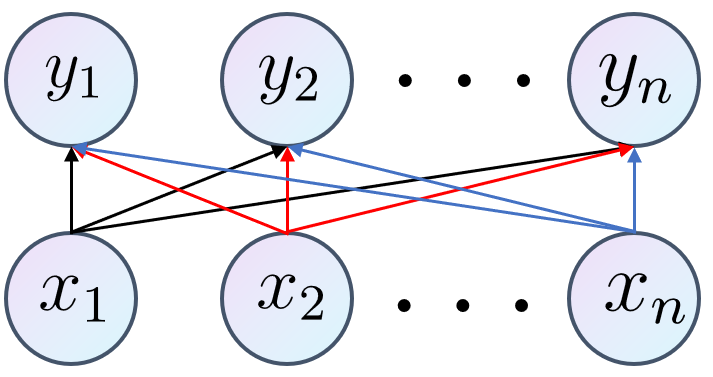
Let’s first see an important example. In fully connected layers, one input neuron sends information (i.e., multiplied by weights) to every output neuron. Denote \(w_{ji}\) as the weight from \(x_i\) to \(y_j\). Then for every output neuron (e.g., \(y_j\)), it accepts the information sent by every input neuron:
$$ y_{j}= \sum\limits_{i} w_{ji} x_{i} \tag{5.1} $$
Then the partial derivative of \(y_j\) with respect to \(x_i\):
$$ \frac{\partial y_j}{\partial x_{i}}= w_{ji} \tag{5.2} $$
Let’s see another example. Comes from Bishop-Pattern-Recognition-and-Machine-Learning-2006
And we can represent it by the computational graph below.
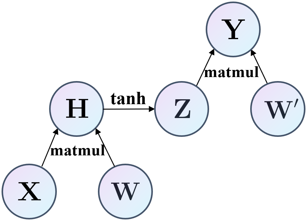
And we can perform a forward propagation according to the computational graph.
where
$$ f(h) = \tanh(h) = \frac{e^h - e^{-h}}{e^h + e^{-h}} \tag{5.6} $$
A useful feature of this activation is that its derivative can be expressed in a particularly simple form:
$$ f’(h) = 1 - f(h)^2 \tag{5.7} $$
The error function can be mean squared errors:
$$ E(\mathbf{w}) = \frac{1}{2} \sum\limits_{k}(y_{k}- \hat{y}_k)^2 \tag{5.8} $$
If we want to update the parameters, we need first to compute the partial derivative of \(E(\mathbf{w})\) with respect to them.
$$ \frac{\partial E(\mathbf{w})}{\partial w_{kj}^{(2)}} = \frac{\partial E(\mathbf{w})}{\partial y_{k}} \frac{\partial y_k}{\partial w_{kj}^{(2)}} = (y_{k}- \hat{y}_k)z_{j} \tag{5.9} $$
$$ \begin{align} \frac{\partial E(\mathbf{w})}{\partial w_{ji}^{(1)}} &= \frac{\partial E(\mathbf{w})}{\partial h_{j}}\frac{\partial h_j}{\partial w_{ji}^{(1)}} = \left(\frac{\partial E(\mathbf{w})}{\partial z_{j}} \frac{\partial z_j}{\partial h_j}\right)x_{i} \tag{5.10} \end{align} $$
$$ \frac{\partial E(\mathbf{w})}{\partial z_j} = \sum\limits_{k}\frac{\partial E(\mathbf{w})}{\partial y_{k}}\frac{\partial y_k}{\partial z_{j}}= \sum\limits_{k} (y_{k}- \hat{y}_{k}) w_{kj}^{(2)}\tag{5.11} $$
\(\text{Remark.}\) \(z_j\) can send information to all the output neurons (e.g., \(y_k\)), thus we need to sum over all the derivatives with respect to \(z_j\).
Substituting \(\text{(4.11)}\) into \(\text{(4.10)}\) we obtain
6. Interpretation
Recall the Taylor approximation of the two variables function:
$$ f(x, y) = f(x_0, y_0) + f_x (x- x_0) + f_y(y-y_0) \tag{6.1} $$
\(\text{Remark.}\) \((x, y)\) needs to be close to \((x_0, y_0)\), otherwise the approximation can fail.
We can transform \(\text{(5.1)}\) into \(\text{(5.3)}\):
If we apply \(\text{(5.3)}\) in the example above, we can obtain
$$ \Delta E(\mathbf{w}) = \nabla_{\mathbf{w}}E(\mathbf{w}) \Delta \mathbf{w} \tag{6.4} $$
From another perspective, a small change in the parameters will propagate into a small change in object function by getting multiplied by the gradient.
To summarize, back-propagation allows information to flow backwards through the network. This information can tell the model a small change in one particular parameter can result in what change in the object function. And gradient descent can use this information to adjust the parameters for optimizing the object function.